Blog Index — Rolling View — RSS
[link—standalone]Lately I've been getting back into film photography. Some years ago I took a fair number of medium format pictures using a Holga pinhole camera. I never digitized any of my negatives, mostly due to the lack of a decent scanner. I still lack a proper scanner, having only a sub-par Brother model meant for documents. However, I may be able to use a few mathematical tricks to make it work far past its intended potential.
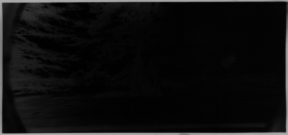
As seen in my first scan, the main problem is I can't control the exposure time on my scanner and negatives end up much too dark. While some information can be recovered by correcting the contrast and gamma of each image, this is overwhelmed by the noise produced by the scanner. Moreover, I was lazy so the film was obscured by dust, hairs, and fingerprints. Fortunately, the random noise can be removed by averaging multiple scans. However, I also wanted to try removing various sources of systematic noise (i.e., prints, hairs, film imperfections). Ultimately, I took 125 scans of the negative in four different positions on the scanner bed, each with their own imperfections. After reading each image into Matlab, I corrected the contrast, gamma, and registered each image to align differences in position and rotation.
img = zeros(2692,5738,125);
for i = 1:125
    % read in scans and correct gamma and contrast limits
    img(:,:,i) = 1-mat2gray(double(imread(['Image_',num2str(i),'.bmp'])));
    img(:,:,i) = imadjust(img(:,:,i),[0.5, 1],[],10);
end

% register images, allowing for rotation and translation
mkdir Registered % directory for registered images
regImg = zeros(2692,5738,125);
[optimizer, metric] = imregconfig('monomodal'); % assume similar brightness and contrast
optimizer.MaximumIterations = 1000; % increase iterations
regImg(:,:,27)=img(:,:,27); % reference image

idx = [1:26, 28:125];
for i=1:length(idx)
    regImg(:,:,i) = imregister(img(:,:,i), img(:,:,27), 'rigid', optimizer, metric);
end

meanImg = mean(regImg,3);
figure; % display mean image
imshow(meanImg,[]);

The end result is pretty rough. However, we can remove the noise produced by the scanner by taking the average of each pixel across all scans.
However, two sources of noise still remain. The various hairs and fingerprints present in the different scans have to be removed. Second, regular vertical lines are present throughout the negative. While these would not be visible in a proper scan, the increased image contrast has made them more present. While the fingerprints will be difficult to address, the lines are regular and can be removed my moving the image into the frequency domain.
ft=fftshift(fft2(meanImg));
amp=abs(ft);
figure;
imagesc(log(amp));
axis image;

As seen above, a strong horizontal line is present throughout the frequency spectra of our image, representing the regular pattern of vertical lines. By removing these frequencies, we should also remove the lines without affecting the rest of our image. So, we will need a function to filter out frequencies ±2° from vertical. As the lines are closely spaced, we don't need to filter out low frequencies, only those above 200 cycles/image.
function thefilter = ofilter(oLow,oHigh,dim);
    % a bandpass filter of size dim that passes orientations between oLow and oHigh
    % horizontal and vertical are 0 and 90 degrees
    t1 = ((0:dim-1)-floor(dim/2))*(2/(dim));
    [t1,t2] = meshgrid(t1,t1);
    a=atan2(t1,t2)*180/pi;
    t1=t1.*t1+t2.*t2;
    clear t2
    a=mod(a,180);
    oLow=mod(oLow,180);
    oHigh=mod(oHigh,180);
    thefilter=ones(size(t1));
    if oHigh>=oLow
        d=find((a=oHigh) & t1>0); % find out-of-band frequencies
    else
        d=find((a=oHigh) & t1>0); % find out-of-band frequencies
    end
    if ~isempty(d)
        thefilter(d)=zeros(size(d));
    end
end

function thefilter = bpfilter(lowf,highf,dim);
    % a bandpass filter of size dim that passes frequencies between lowf and highf
    dc=[round(dim/2)+1,round(dim/2)+1];
    thefilter=zeros(dim,dim);
    dx=1:dim;dx=dx-dc(1);
    for yk=1:dim
        dy=dc(2)-yk;
        d=sqrt(dx.*dx + dy*dy);
        val1=find((d > lowf)&(d < highf));
        thefilter(yk,val1)=ones(1,length(val1));
    end
end

function thefilter=filter2d(lowf,highf,orient1,orient2,dim);
    % combines ofilter and bpfilter to pass frequencies between lowf and highf
    % and orientations between orient1 and orient2
    thefilter=bpfilter(lowf,highf,dim);
    temp=ofilter(orient1,orient2,dim);
    thefilter=thefilter.*temp;
    return;
end
Given the function filter2d, we can apply it to each image to remove all frequencies above 200 cycles/image that are within 2° of vertical.
thefilter = filter2d(200,5738,88,92,5738);
thefilter = 1-thefilter(1524:4215,:);

for i=1:125
    ft=fftshift(fft2(regImg(:,:,i)));
    amp=abs(ft);
    phase=angle(ft);
    r=size(amp,1);c=size(amp,2);
    dc=[round(r/2)+1,round(c/2)+1];
    dcAmp=amp(dc(1),dc(2));
    amp = amp.*thefilter;
    ft = amp.*exp(sqrt(-1)*phase);
    filtImg(:,:,i)=real(ifft2(fftshift(ft)));
end
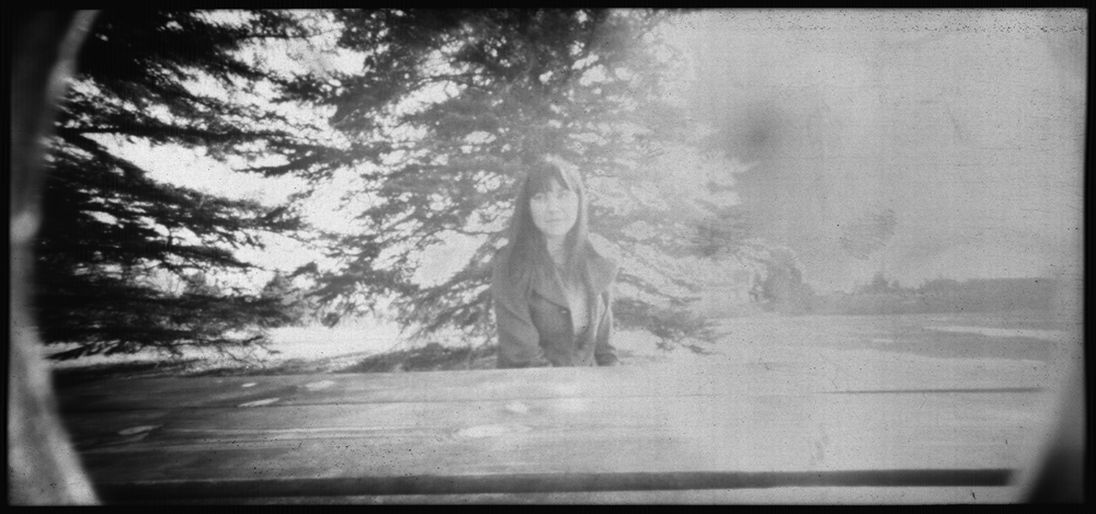
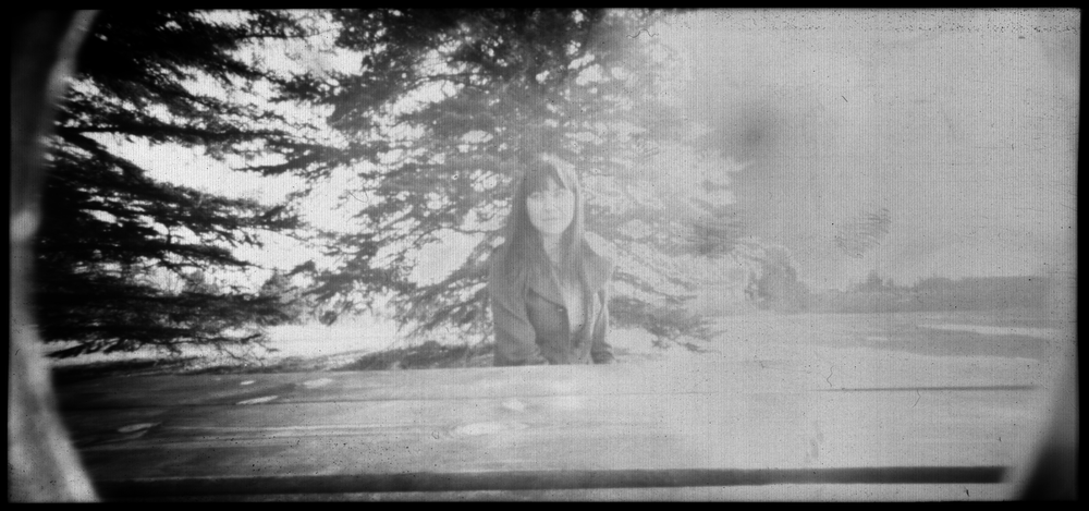
Finally! We have removed the lines and are one step closer to having a clean picture. All that remains is to remove the various hairs and fingerprints present in each image. Fortunately, the position of these flaws varied between scans. I wiped down the negative, removing some prints and causing others to be deposited. Since presence or absence of these flaws are independent of the image, we can use independent component analysis (ICA) to isolate them and subtract them from our average image. The FastICA package is one of the best implementations of ICA.
filtImg=filtImg(59:2643,50:5678,:); % to avoid exceeding RAM capacity
[rows, columns, scans] = size(filtImg);
pcaArray = reshape(filtImg, rows * columns, scans)'; % reshape array for ICA
mu = mean(pcaArray,1); % the average image, ICA automatically subtracts this
[icasig, A] = fastica(pcaArray, 'lastEig', 8, 'numOfIC', 8); % take first 8 components
baseCase = mean(A(76:125,:),1); % scores for fingerprint-free images

% positive and negative parts of the first three components
ICAp1 = icasig(1,:); ICAp1(ICAp1 < 0) = 0;
ICAm1 = -icasig(1,:); ICAm1(ICAm1 < 0) = 0;
ICAp2 = icasig(2,:); ICAp2(ICAp2 < 0) = 0;
ICAm2 = -icasig(2,:); ICAm2(ICAm2 < 0) = 0;
ICAp3 = icasig(3,:); ICAp3(ICAp3 < 0) = 0;
ICAm3 = -icasig(3,:); ICAm3(ICAm3 < 0) = 0;
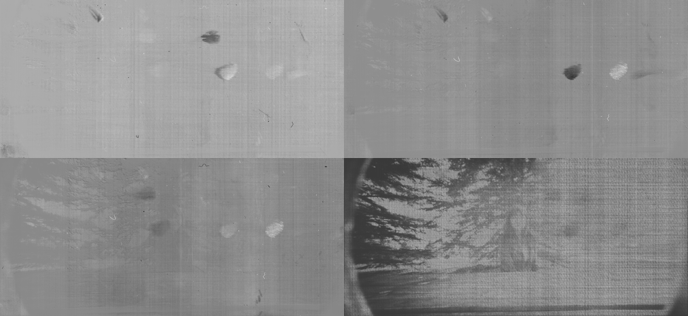
As seen above, ICA has isolated all the fingerprints and hairs that obscured our image within the first three independent components. Since all scans had defects, the absence of a flaw in one image implies the presence of another elsewhere. Therefore, each component captures both the presence (positive values & lighter pixels) and absence (negative values & darker pixels) of various features. As we want to make an image that contains none of these flaws, we separate the positve and negative values of each component.
All that remains is to find the ideal combination of component weights that removes all blemishes from the average image (mu). My approach was to generate random weights for two sets of components, add these to the average image, and indicate which looked better. It is a bit hacky, but a few iterations resulted in an image that looked half decent.
WeightArr = [rand(1,2).* 0.026 - 0.013; ...
    rand(1,2).* 0.016 - 0.008; ...
    rand(1,2).* 0.0608 - 0.0304];
for i = 1:100
    tmpArr = [rand(1,2).* 0.026 - 0.013; ...
        rand(1,2).* 0.016 - 0.008; ...
        rand(1,2).* 0.0608 - 0.0304];
    figure('units','normalized','outerposition',[0 0 1 1]);
    subplot(2,1,1)
    imshow(reshape((mu+ICAp1.*WeightArr(1,1)+ICAp2.*WeightArr(2,1)+ICAp3 ...
    .*WeightArr(3,1)+ICAm1.*WeightArr(1,2)+ICAm2.*WeightArr(2,2)+ICAm3 ...
    .*WeightArr(3,2))',rows,columns),[]);
    subplot(2,1,2)
    imshow(reshape((mu+ICAp1.*tmpArr(1,1)+ICAp2.*tmpArr(2,1)+ICAp3 ...
    .*tmpArr(3,1)+ICAm1.*tmpArr(1,2)+ICAm2.*tmpArr(2,2)+ICAm3 ...
    .*tmpArr(3,2))',rows,columns),[]);
    drawnow;
    w = waitforbuttonpress;
    if w
        WeightArr = tmpArr;
    end
end

imwrite(uint16(mat2gray(reshape((mu+ICAp1.*WeightArr(1,1)+ICAp2.*WeightArr(2,1) ...
+ICAp3.*WeightArr(3,1)+ICAm1.*WeightArr(1,2)+ICAm2.*WeightArr(2,2)+ICAm3 ...
.*WeightArr(3,2) )', rows, columns) ).*65535),'FinalImg.tif');
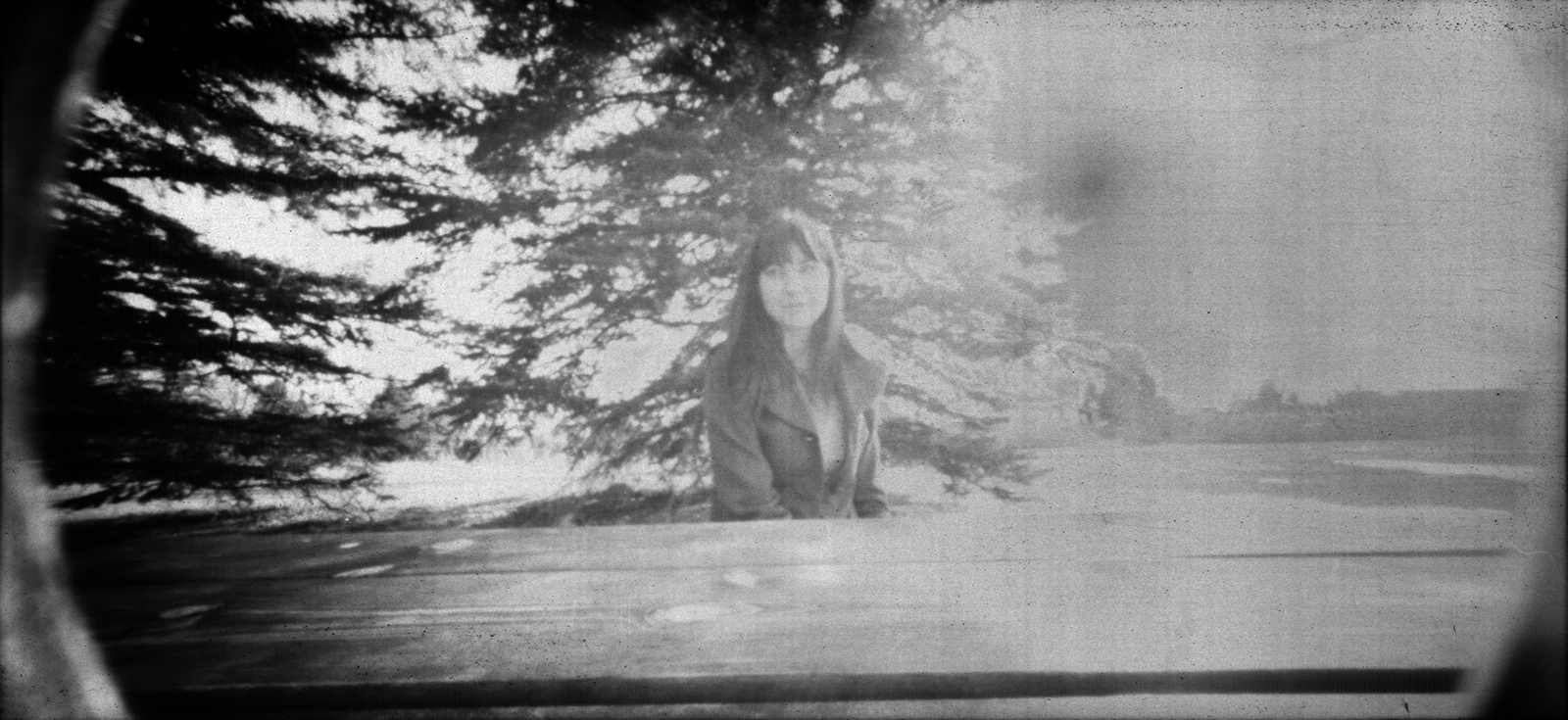
And here it is, the final image. While it still could use a lot of work, the end result is a far cry from what my scanner initially produced. However, the main lesson is that I should probably buy a better scanner.